
0. Introduction
Dataset: Heart Disease UCI (UCI 데이터)
이 데이터셋은 총 303명의 환자의 의료 정보와 심장병 발병 여부를 담고 있는 데이터셋입니다. 총 13개의 입력변수와 1개의 타겟변수로 구성되어 있습니다. 변수를 살펴보면:
- age: 환자의 나이
- sex: 성별 (1=남성, 0=여성)
- cp: 가슴 통증의 유형 (0-3)
- trestbps: 혈압
- chol: 콜레스테롤 수치 (mg/dl)
- fbs: 공복혈당수치가 120ml/dl을 초과하는지 여부 (1 = true, 0=false)
- restecg: 심전도 결과 (0=정상, 1=ST-T wave, 2=좌심실비대)
- thalach: 최대 심박수
- exang: 운동 유발성 협심증 여부 (1=yes, 0=no)
- oldpeak: ST분절 하강
- slope: the slope of the peak exercise ST segment (0-2)
- ca: 형광투시로 칠해진 주요 혈관의 개수(0-3)
- thal: 1 = normal; 2 = fixed defect; 3 = reversable defect
- num (타겟변수): 심장병 여부 (0=no disease, 1=disease)
Heart 데이터셋을 활용하여 R에서 제공하는 Decision Tree 패키지 4개로 Classsification tree를 만들어 보겠습니다. 모델마다 가지치기를 하기 전과 후의 성능을 비교해보고 패키지 간 성능도 비교해보겠습니다.
학습에 앞서 전체 데이터셋을 임의로 200개의 training set과 103개의 validation set으로 나눴습니다.
# Load the data & Preprocessing
heart <- read.csv("heart (4).csv")
input.idx <- c(1:13)
target.idx <- 14

heart.input <- heart[,input.idx]
heart.target <- as.factor(heart[,target.idx])

heart.data <- data.frame(heart.input, heart.target)

#Separate Training and Test Dataset
set.seed(28352)
trn_idx <- sample(1:length(heart.target), round(0.66*length(heart.target)))
trnInputs <- heart.input[trn_idx,]
trnTargets <- heart.target[trn_idx]
valInputs <- heart.input[-trn_idx,]
valTargets <- heart.target[-trn_idx]

heart.trn <- heart.data[trn_idx,]
heart.tst <- heart.data[-trn_idx,]
1. “tree” Package
먼저 tree 패키지를 사용했습니다.
1.1. Tree before pruning
가지치기를 하기 전과 후를 비교하기 위해 우선 가지치기를 하지 않은 모델을 만들었습니다.
1.1.1. Classification Tree 학습 결과 및 해석
위에서 준비한 training set으로 “tree”package를 사용해 Classification Tree를 학습했습니다.
# Q1. Classification and Regression Tree (CART) -------------------------------
# Training the tree
heart.model <- tree(heart.target ~ ., heart.trn)
summary(heart.model)
# Plot the tree
plot(heart.model)
text(heart.model, pretty = 2)
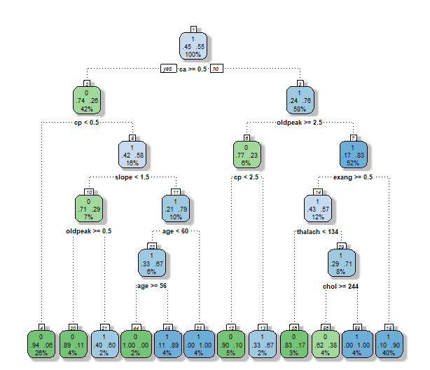
결과는 다음과 같습니다.
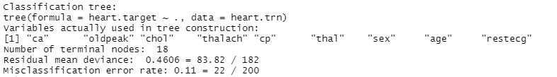
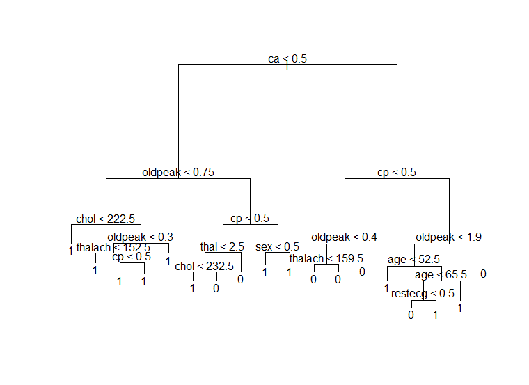
- 우선 Root node에서는 ca가 decision variable로 사용되었습니다. Decision point는 0.5였다. 위에서 쪼개진 왼쪽 노드는 다시 oldpeak이 0.75보다 작은지를 기준으로 나뉘었고 오른쪽 노드는 cp가 0.5보다 작은지를 기준으로 나뉘었습니다.
- 이렇게 쪼개기를 반복한 결과 ca, oldpeak, chol, cp, thal, sex, thalach, age 등의 변수를 사용하여 18개의 leaf node가 생성되었습니다.
- ca 변수가 가장 먼저 decision variable로 선택된 것으로 보아 매우 중요한 변수라고 판단됩니다.
1.1.2. Validation Dataset에 대한 분류 성능
위에서 학습한 tree를 pruning하지 않은 상태에서 validation set으로 분류 성능을 평가했습니다.
#Validation before pruning
# Prediction
haert.prey <- predict(heart.model, heart.tst, type = "class")
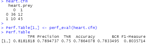
heart.cfm <- table(heart.tst$heart.target, haert.prey)
heart.cfm
Perf.Table[1,] <- perf_eval(heart.cfm)
Perf.Table
Confusion Matrix와 성능 지표는 다음과 같습니다.
| 구분 | TPR | Precision | TNR | Accuracy | BCR | F1-Measure |
| Before Pruning | 0.8363636 | 0.779661 | 0.7291667 | 0.7864078 | 0.780928 | 0.8070175 |
- Accuracy는 0.7864이었습니다.
- TPR은 0.8364였고 이는 실제 환자들 중에서 83.64%가 제대로 예측되었음을 의미합니다.
- TNR은 0.7292로 이것은 실제 환자가 아닌 사람들 중에서 72.92%가 제대로 분류되었음을 나타냅니다.
- Precision은 0.7797로 환자라고 분류했을 때 그 중 77.97%가 실제 환자였다는 것을 나타냅니다.
- Accuracy의 단점을 보완한 BCR과 F1을 살펴보았을 때 각각 0.7809와 0.8070이라는 비교적 높은 수치가 계산되었습니다. Tree를 Pruning 하지 않아 과적합된 tree가 생성되었기 때문에 Pruning을 수행하면 성능이 향상될 것으로 예상됩니다.
1.2. Tree After Pruning
1.2.1. 수행 결과 및 해석
앞에서 생성한 Tree에 대해서 leaf node의 개수에 따른 deviance의 증감을 살펴보았습니다.
# Q2.Find the best tree
set.seed(12345)
heart.model.cv <- cv.tree(heart.model, FUN = prune.misclass)

# Plot the pruning result
plot(heart.model.cv$size, heart.model.cv$dev, type = "b")
heart.model.cv
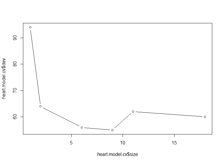
| size | 18 | 11 | 9 | 6 | 2 | 1 |
|---|---|---|---|---|---|---|
| deviance | 60 | 62 | 55 | 56 | 64 | 94 |
- Leaf node가 9개에서 11개로 증가할 때 deviance가 오히려 커지는 것을 알 수 있습니다. 따라서 최적의 leaf node 개수는 9개라고 판단했습니다
Leaf node가 9개가 되도록 가지치기를 수행했습니다.
# Select the final model
heart.model.pruned <- prune.misclass(heart.model, best = 9)
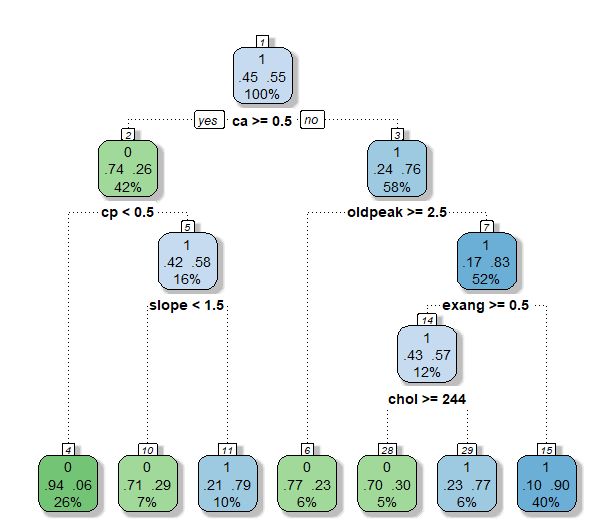
plot(heart.model.pruned)
text(heart.model.pruned, pretty = 1)
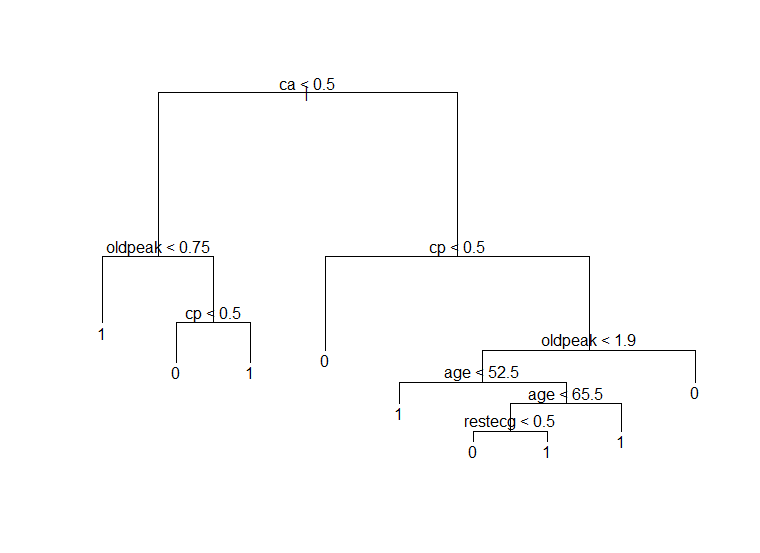
- Pruning을 하자 18개였던 terminal node가 9개로 줄어들었습니다.
- Pruning 전에는 ca로 우선 쪼개진 후 왼쪽 노드에서 oldpeak, chol, thalach, cp, thal, sex 등의 변수가 사용되었지만 pruning 후에는 oldpeak과 cp만이 사용되었습니다.
- 오른쪽 노드에서는 pruning 전 cp, oldpeak, thalach, age, restecg 변수가 사용되었지만 pruning 후에는 thalach 변수를 사용하지 않았습니다.
1.2.2. Validation dataset에 대한 분류 성능
Pruning 된 tree에 대해 validation set으로 분류 성능을 계산해보았다.
heart.prey <- predict(heart.model.pruned, heart.tst, type = "class")
heart.cfm <- table(heart.tst$heart.target, heart.prey)
heart.cfm

Perf.Table[1,] <- perf_eval(heart.cfm)
Perf.Table
Pruning 전과 비교해서 accuracy는 0.7864로 동일했다. TPR, F1은 각각 감소했고 TNR, Precision, BCR은 살짝 증가했다. TPR이 감소했다는 것은 환자라고 예측한 사람들 중에서 실제 환자가 아니었던 비중이 커졌음을 의미하며 TNR이 증가했다는 것은 환자가 아니라고 예측한 사람들 중에서 실제 환자가 아니었던 비중이 커졌음을 의미한다. 과적합된 tree를 pruning을 통해 개선했기 때문에 몇몇 지표들이 증가한 것으로 보인다.
2. “rpart” Package
2.1. “rpart”패키지의 옵션
“rpart” 패키지가 Classification Tree를 학습할 때 사용자가 지정할 수 있는 옵션의 종류와 의미는 다음과 같습니다.
Rpart 함수: rpart(formula, data, weights, subset, na.action = na.rpart, method, model = FALSE, x = FALSE, y = TRUE, parms, control, cost, …)
| 옵션 | 설명 |
|---|---|
| subset | 데이터에서 특정 행만을 선택해 사용하도록 한다. |
| na.action | y에 missing value가 있을 때 default action은 해당 관측치를 제거하지만, 이 옵션 사용시 제거하지 않는다. |
| method | poisson: y 컬럼이 2개일 때 사용한다. class:y가 factor형 변수일 때 사용한다. exp: y가 survival object일 때 사용한다. anova:y가 위의 조건에 해당하지 않을 때 사용한다. method를 선택하지 않을 시 적당한 method를 추측하여 사용한다. |
| X | 결과의 x matrix 사본을 저장한다. |
| y | 결과의 dependent variable을 저장한다. |
| Parms | Splitting function의 옵션을 지정한다. Anova splitting은 파라미터가 없다. Poisson splitting은 coefficient of variation of the prior distribution on the rates를 파라미터로 가지며 default는 1이다. Exponential splitting은 Poisson과 동일한 파라미터를 가진다 Classification splitting의 경우, vector of prior probabilities, loss matrix, splitting index 등을 가질 수 있다. Loss matrix는 반드시 대각선에 0을 가지고 있으며 나머지는 양수를 가져야 한다. Splitting index는 gini 혹은 information을 선택할 수 있다. Default는 gini이다. |
| control | Rpart 알고리즘의 세부적인 부분을 컨트롤 한다. minsplit: split하기 전 노드에 있어야할 관측치의 최소값 minbucket: leaf node에 있어야할 관측치의 최소값 (minbucket을 minsplit/3으로 설정하는 것이 적절하다.) cp: complexity parameter이다. maxdepth: 최종 tree의 최대 depth (root node는 0으로 카운트된다.) |
2.2 옵션의 변화에 따른 Classification Tree들의 차이점 및 Best Model 선정
옵션들을 변화시켜가며 생성된 classification tree들의 차이점을 살펴보고 이 중에서 best model을 선정했습니다.
- 바꾼 옵션들은 splitting index, minsplit, maxdepth였습니다. Minsplit이 결정되면 minbucket은 minsplit/3으로 설정되므로 따로 변화시키지 않았습니다. Minsplit과 maxdepth는 모두 tree의 depth를 결정하므로 동시에 고려하지 않았습니다.
2.2.1 Splitting index = gini, entropy
Splitting index를 gini와 entropy를 사용해 각각 tree를 구축했습니다.
#Q3. rpart_____________________________________________________________________________________________
#2.2.1 gini and entropy
#gini
heart.rpart <- rpart(heart.target ~., data = heart.trn, method='class')
fancyRpartPlot(heart.rpart)
# Prediction
heart.prey <- predict(heart.rpart, heart.tst, type = "class")
heart.cfm <- table(heart.tst$heart.target, heart.prey)
heart.cfm
Perf.Table<- rbind(Perf.Table, perf_eval(heart.cfm))
Perf.Table

#entropy
heart.rpart <- rpart(heart.target ~., data = heart.trn, method='class', parms = list(split="entropy"))
fancyRpartPlot(heart.rpart)
# Prediction
heart.prey <- predict(heart.rpart, heart.tst, type = "class")
heart.cfm <- table(heart.tst$heart.target, heart.prey)
heart.cfm
Perf.Table<- rbind(Perf.Table, perf_eval(heart.cfm))
Perf.Table
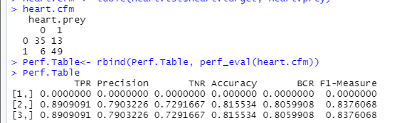
결과는 다음과 같다.

| 구분 | TPR | Precision | TNR | Accuracy | BCR | F1-Measure |
|---|---|---|---|---|---|---|
| Gini | 0.8909091 | 0.7903226 | 0.7291667 | 0.815534 | 0.8059908 | 0.8376068 |
| Entropy | 0.8909091 | 0.7903226 | 0.7291667 | 0.815534 | 0.8059908 | 0.8376068 |
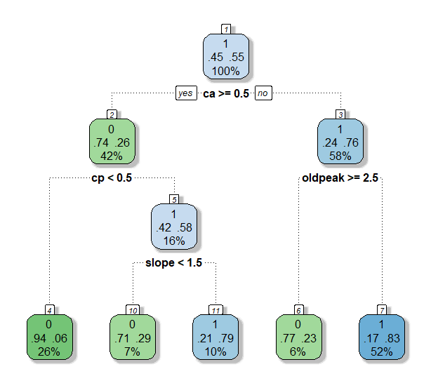
- 두가지 옵션 모두 동일한 tree가 구축되었고 performance measure 역시 일치했다.
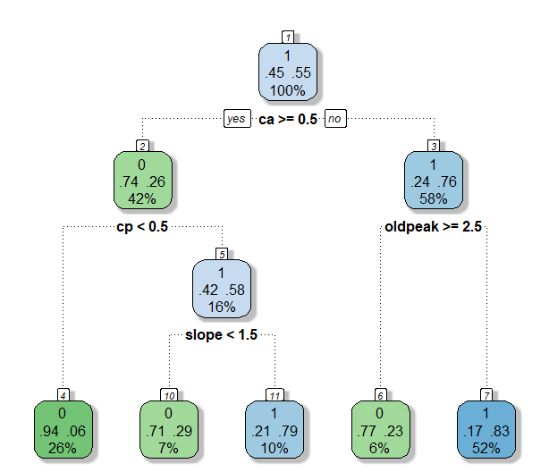
- 5번의 splitting을 통해 7개의 leaf node가 생성되었다. 맨 처음 사용된 변수는 ca로 tree 패키지에서 생성되었던 tree와 동일했다.
- Leaf node에서 각 클래스의 비율을 살펴보면 모두 70% 이상으로 impurity가 비교적 낮음을 알 수 있다. TPR은 0.89로 매우 높은 반면 TNR은 0.73으로 살짝 낮았는데, 이 때문에 accuracy는 0.81이 계산되었다. BCR과 F1은 각각 0.8060과 0.8376으로 높은 값을 나타냈다.
2.2.2 minsplit = 10, 20, 30
다음은 minsplit을 10, 20, 30으로 변화시켜가며 tree를 구축했습니다. 위에서 gini index와 entorpy의 차이가 없었으므로 여기서는 gini index만을 사용했습니다.
#2.2.2 minsplit = 10, 20, 30
# Performance table
Perf.Table <- matrix(0, nrow = 1, ncol = 6)
colnames(Perf.Table) <- c("TPR", "Precision", "TNR", "Accuracy", "BCR", "F1-Measure")

for (i in c(10, 20, 30)){
  heart.rpart <- rpart(heart.target ~., data = heart.trn, method='class',control = rpart.control(minsplit = i) )
  fancyRpartPlot(heart.rpart)

  # Prediction
  heart.prey <- predict(heart.rpart, heart.tst, type = "class")
  heart.cfm <- table(heart.tst$heart.target, heart.prey)
  heart.cfm

  Perf.Table<- rbind(Perf.Table, perf_eval(heart.cfm))
  Perf.Table

}
Perf.Table

| 구분 | TPR | Precision | TNR | Accuracy | BCR | F1-Measure |
|---|---|---|---|---|---|---|
| minsplit = 10 | 0.8727273 | 0.8 | 0.75 | 0.815534 | 0.8090398 | 0.8347826 |
| minsplit = 20 | 0.8909091 | 0.7903226 | 0.7291667 | 0.815534 | 0.8059908 | 0.8376068 |
| minsplit = 30 | 0.9090909 | 0.7462687 | 0.6458333 | 0.7864078 | 0.7662384 | 0.8196721 |
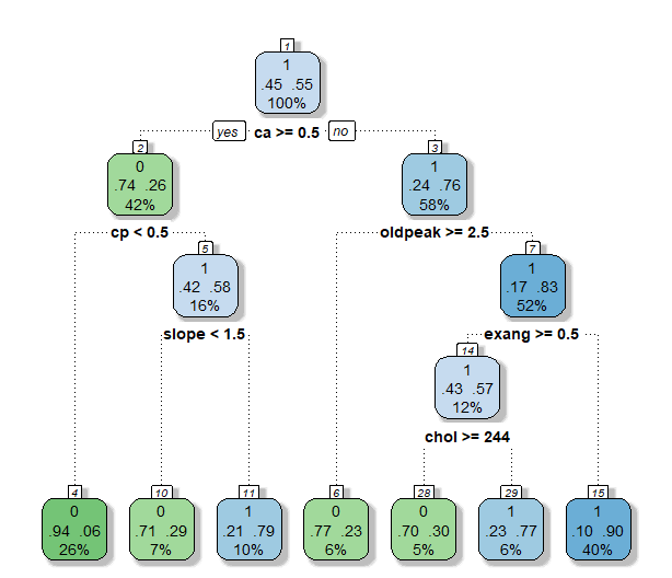
- Minsplit을 10으로 설정했을 때는 보다 복잡한 tree가 구축되었다. 11번의 split이 있었고, 12개의 terminal node가 생성되었다. TPR은 다른 minsplit 옵션에 비해 낮은 값을 보였지만 F1을 제외한 나머지 measure에 대해선 가장 좋은 성능을 보였다.
- Minsplit을 20으로 설정했을 때는 보다 간단한 tree가 구축되었다. 6번의 split이 있었고, 7개의 terminal node가 생성되었다. 각 terminal node의 비율을 살펴보면 impurity가 비교적 낮음을 알 수 있다. 다른 모델들과 비교했을 때, 가장 높은 F1값을, 나머지 measure에 대해서는 모두 2위를 차지했다. Minsplit이 10일 때 보다 node가 줄어들면서 성능이 약간 떨어졌지만 minsplit이 10일 때와 꽤 유사한 값을 보였다.
- 마지막으로 minsplit이 30일 때는 4번의 split으로 5개의 leaf node가 생성되었다. TPR은 다른 모델들에 비해 높았으나 나머지 measure에서 가장 안 좋은 성능을 보였다. 제대로 분류를 하기에 leaf node의 개수가 너무 적은 것으로 보인다.
2.2.3 maxdepth = 4, 5, 6
#2.2.3 maxdepth = 4, 5, 6
# Performance table
Perf.Table <- matrix(0, nrow = 1, ncol = 6)
colnames(Perf.Table) <- c("TPR", "Precision", "TNR", "Accuracy", "BCR", "F1-Measure")

for (i in c(4, 5, 6)){
  heart.rpart <- rpart(heart.target ~., data = heart.trn, method='class',control = rpart.control(maxdepth = i) )
  fancyRpartPlot(heart.rpart)

  # Prediction
  heart.prey <- predict(heart.rpart, heart.tst, type = "class")
  heart.cfm <- table(heart.tst$heart.target, heart.prey)
  heart.cfm

  Perf.Table<- rbind(Perf.Table, perf_eval(heart.cfm))
  Perf.Table

}
Perf.Table

| 구분 | TPR | Precision | TNR | Accuracy | BCR | F1-Measure |
|---|---|---|---|---|---|---|
| maxdepth = 3 | 0.9090909 | 0.7462687 | 0.6458333 | 0.7864078 | 0.7662384 | 0.8196721 |
| maxdepth = 4 | 0.8909091 | 0.7903226 | 0.7291667 | 0.815534 | 0.8059908 | 0.8376068 |
| maxdepth = 5 | 0.8909091 | 0.7903226 | 0.7291667 | 0.815534 | 0.8059908 | 0.8376068 |
- Maxdepth를 3으로 설정했을 때에는 minsplit이 30일때와 같은 결과를 나타냈다. 4번의 split으로 5개의 leaf node가 생성되었다. TPR은 세 모델들 중에서 가장 높았지만 다른 measure들에서는 가장 성능이 떨어졌다. 특히 TNR이 0.6458로 계산되어 환자가 아닌 사람들을 분류할 때 성능이 좋지 않았다.
- Maxdepth가 4일때와 5일때는 모두 minsplit이 20일 때와 같은 tree가 생성되었다. Maxdepth가 3일 때 보다 살짝 복잡한 tree가 구축되었다. 6번의 split이 있었고, 7개의 terminal node가 생성되었다. 각 terminal node의 비율을 살펴보면 impurity가 비교적 낮음을 알 수 있다. Maxdepth를 3으로 설정한 모델과 비교했을 때, TPR을 제외하면 모든 measure에서 높은 성능을 보였다. TPR 역시 크게 차이나지 않았다.
2.2.4 Best Model 선정
| 구분 | TPR | Precision | TNR | Accuracy | BCR | F1-Measure |
|---|---|---|---|---|---|---|
| Gini | 0.8909091 | 0.7903226 | 0.7291667 | 0.815534 | 0.8059908 | 0.8376068 |
| Entropy | 0.8909091 | 0.7903226 | 0.7291667 | 0.815534 | 0.8059908 | 0.8376068 |
| minsplit = 10 | 0.8727273 | 0.8 | 0.75 | 0.815534 | 0.8090398 | 0.8347826 |
| minsplit = 20 | 0.8909091 | 0.7903226 | 0.7291667 | 0.815534 | 0.8059908 | 0.8376068 |
| minsplit = 30 | 0.9090909 | 0.7462687 | 0.6458333 | 0.7864078 | 0.7662384 | 0.8196721 |
| maxdepth = 3 | 0.9090909 | 0.7462687 | 0.6458333 | 0.7864078 | 0.7662384 | 0.8196721 |
| maxdepth = 4 | 0.8909091 | 0.7903226 | 0.7291667 | 0.815534 | 0.8059908 | 0.8376068 |
| maxdepth = 5 | 0.8909091 | 0.7903226 | 0.7291667 | 0.815534 | 0.8059908 | 0.8376068 |
- 모델들의 성능을 살펴볼 때, precision이 가장 중요하다고 생각했다. 환자가 아닌 사람을 환자라고 하는 위험보다 환자를 환자가 아니라고 하는 위험이 훨씬 크기 때문이다. 따라서 실제 환자 중에서 환자라고 제대로 예측한 비율인 precision이 가장 중요한 measure라고 보았을 때, minsplit을 10으로 설정한 모델이 best model이라고 선정했다. 다른 모델들과 비교해서도 크게 차이나지 않는 TPR을 가졌고, TNR 역시 다른 모델들에 비해 가장 높은 0.75였다. Accuracy는 다른 모델들과 동일하게 1위를 차지했다. BCR 역시 가장 높은 값을, F1은 둘째로 높은 값을 보였기 때문에 Best model로 선정함이 타당하다.